반응형
ggplot 그래프를 3D로 랜더링 해보자
오늘은 rayshader라는 R 패키지에 대하여 알아보도록 하자.
ray는 광선을 의미하는데, 게임에서 좀 더 현실적인 효과를 얻기위하여 픽셀별로 빛의 세기를 렌더링하는 방법을 raytracing이라고 한단다. 이런 ray tracing기법을 이용해서? ggplot 그래프를 3d로 바꿔주는 패키지가 있다. 바로 rayshader라는 R 패키지. 이름에서 느껴지다시피 빛을 생각해서 그림자를 그려준다는 의미로 이름을 지은것 같다.
예제 1
다음의 R코드를 보자. 유명한 ggplot2의 diamonds 데이터 셋에 접근해서 등고선 그래프를 다이아몬드 투명도에 따라서 그린 그래프이다.
library(ggplot2)

gg <- ggplot(diamonds, aes(x, depth)) +
    stat_density_2d(aes(fill = stat(nlevel)),
                    geom = "polygon",
                    n = 100, bins = 10, contour = TRUE) +
    facet_wrap(clarity~.) +
    scale_fill_viridis_c(option = "A")
gg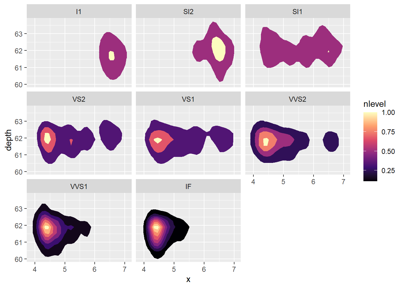
요렇게 만든 gg 오브젝트를 rayshader패키지의 plot_gg함수에 다음과 넣으면 3d 렌더링 된 함수를 만날 수 있다.
plot_gg(gg, multicore = TRUE,
        width = 5, height = 5, scale = 250)
예제 2
두번째 예제는 지도을 그리는 예제이다.
# built-in palettes:
# “imhof1”, “imhof2”, “imhof3”, "imhof4“, ”desert“, ”bw“, ”unicorn".

montereybay %>%
    sphere_shade(zscale = 10, texture = "imhof1") %>%
    add_shadow(ray_shade(montereybay, zscale = 50)) %>%
    add_shadow(ambient_shade(montereybay, zscale = 50)) %>%
    plot_3d(montereybay, zscale = 50, theta = -45, phi = 45,
            windowsize = c(600,600), zoom = 0.5,
            water = TRUE, waterlinealpha = 1,
            wateralpha = 0.5, watercolor = "lightblue",
            waterlinecolor = "white")
반응형
'R' 카테고리의 다른 글
| [PoliscieR] 정치학과에서 R로 연구하기 (13) | 2021.01.31 |
|---|---|
| Rstudio 시작시 특정 R패키지 실행하기 - .Rprofile 파일에 대하여 (0) | 2021.01.25 |
| Rmd파일로 티스토리 포스트용 html 만들기 (6) | 2021.01.13 |
| R패키지 설치시 00LOCK 폴더 오류해결법 (3) | 2021.01.06 |
| Forward propagation, R 버전 (0) | 2020.07.17 |


댓글